TechOps Examples
Hey — It's Govardhana MK 👋
Welcome to another technical edition.
Every Tuesday – You’ll receive a free edition with a byte-size use case, remote job opportunities, top news, tools, and articles.
Every Thursday and Saturday – You’ll receive a special edition with a deep dive use case, remote job opportunities and articles.
👋 👋 A big thank you to today's sponsor PERFECTSCALE
Cloud native apps need to scale up and down quickly.
But how do you do this with modern Java?
Join Pasha Finkelstein, Developer Advocate at Bellsoft, for a hands-on session where he’ll start with a simple “fat JAR” image and gradually rebuild it for cloud-native performance.
You’ll learn how to:
→ Optimize Java apps for Docker and Kubernetes
→ Cut image size, startup time, and deployment lag
→ Fine-tune performance and resource allocation on K8s
IN TODAY'S EDITION
🧠 Use Case
How Kubernetes Predictive AutoScaling Works
👀 Remote Jobs
Social Discovery Group is hiring a DevOps Engineer
Remote Location: Worldwide
FirstPrinciples is hiring a DevOps / Infrastructure Engineering
Remote Location: Worldwide
📚 Resources
If you’re not a subscriber, here’s what you missed last week.
To receive all the full articles and support TechOps Examples, consider subscribing:
One-time 25% OFF on all annual plans of memberships. Closes Soon.
🧠 USE CASE
How Kubernetes Predictive AutoScaling Works
Traditional autoscaling reacts to what already happened; a surge in requests, CPU usage, or queue lengt; by scaling pods after the spike. This reactive model is simple but not ideal in situations when metric data that drive the scaling decision has strong seasonal patterns.
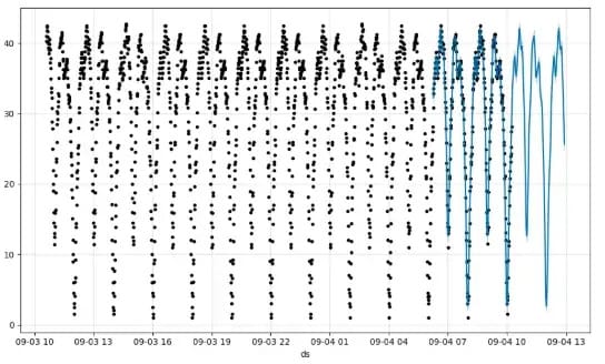
Kedify’s new predictive scaler adds foresight to the process. By applying time series forecasting models like Prophet, Kedify can anticipate future workload changes and adjust scaling before the load hits your infrastructure. The result: smoother performance, fewer cold starts, and smarter resource utilization.
From Reactive to Predictive Scaling
At the beginning there was HPA. HPA can react on CPU or Memory utilization. With traditional KEDA’s scalers, you can plug any metric and react faster then with classical HPA (HTTP requests, length of the message queue, etc.). That works well for most workloads, but some patterns repeat predictably (daily peaks, weekly cycles, monthly cron jobs). Instead of chasing them, Kedify can learn then.
Once enough historical samples are collected, Kedify trains a forecasting model to predict metric values in the near future. These predictions feed directly into autoscaling decisions.
Common forecasting methods considered include:
Moving average and exponential smoothing
ARIMA
Facebook Prophet
LSTM neural networks
Holt-Winters’ method
etc.
Among them, Prophet stands out for its robustness, interpretability, and ability to handle seasonality without heavy tuning.

How the Predictive Model Works
The predictive system continuously collects metric data through Kedify’s integration with KEDA. Once enough data accumulates, the model enters a periodic training and evaluation cycle to maintain accuracy as patterns evolve.
During retraining:
The dataset is split into a train set (90%) and a test set (10%).
The model is trained on the train set and evaluated on the test set using the Mean Absolute Percentage Error (MAPE) metric.
The acceptable MAPE threshold can be configured in the
kedify-predictivetrigger viamodelMapeThreshold.If the model’s error exceeds the threshold, Kedify automatically returns a default value (also defined in the trigger) instead of an unreliable prediction.
This ensures the scaler remains stable and trustworthy, even if patterns change or data becomes noisy. We may use scaling modifiers to ignore the scaler if it returns the default value. Do not expect impossible, not all the data exhibit seasonal patterns and general ML rule of thumb: “garbage in, garbage out” also applies here.
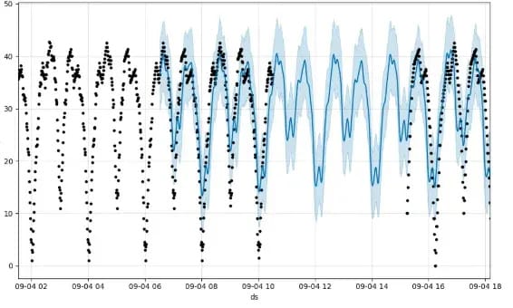
In the visualization below, the light-blue shadow represents the model’s uncertainty bounds. When data collection was interrupted for several hours, the Prophet model still maintained a plausible fit. The widening confidence interval signals increasing uncertainty.

Explainability and Transparency
Although forecasting models can feel like black boxes, Kedify keeps them interpretable. Each model can be decomposed into seasonal and trend components (weekly, monthly, or custom) allowing visual inspection of whether the detected patterns make sense.
This decomposition helps operators trust (or challenge) predictions and fine-tune seasonality parameters as needed.
Introducing the MetricPredictor CRD
Kedify introduces a new Custom Resource Definition: MetricPredictor. It represents the forecasting model and its lifecycle.
apiVersion: kedify.io/v1alpha1
kind: MetricPredictor
metadata:
  name: rabbit
spec:
  source:
    active: true
    keda:
      kind: scaledobject
      name: my-so
      triggerName: rabbit
    retention: 6mo
  model:
    type: Prophet
    defaultHorizon: 5m
    retrainInterval: 6h
    prophetConfig:
      holidays:
        countryCode: US
        strength: 10
      seasonality:
        yearly: "true"
        weekly: "true"
        daily: "true"
        custom:
          name: twoHours
          period: 2h
          fourierOrder: 10
      changepointPriorScale: 0.05
Key points:
sourcedefines where metrics come from — either a liveScaledObjector a one-shot CSV for testing or bootstrapping the model with existing data.modeldefines the forecasting method (Prophet by default) and training cadence.Kedify retrains models automatically on schedule.
Using Predictions in ScaledObjects
Once a MetricPredictor is created and trained, its predictions can be referenced directly in a ScaledObject trigger. This allows Kedify to scale based on forecasted metrics alongside real-time ones.
apiVersion: keda.sh/v1alpha1
kind: ScaledObject
metadata:
  name: my-so
spec:
  triggers:
    - name: rabbit
      type: rabbitmq
      metadata:
        queueName: tasks
        value: "1"
    - name: rabbitFromNearFuture
      type: kedify-predictive
      metadata:
        modelName: default*rabbit
        modelMapeThreshold: "40"
        highMapeDefaultReturnValue: "1"
      targetValue: "1"
  advanced:
    scalingModifiers:
      formula: "(rabbit + rabbitFromNearFuture)/2"
      target: "1"
      metricType: "AverageValue"
Benefits of Predictive Scaling
Reduced reaction lag — the cluster scales before spikes hit.
Improved UX — fewer cold starts and latency dips.
Explainable models — operators can inspect trends and patterns.
Robustness — automatic fallback to defaults when model confidence drops.
Continuous learning — retraining keeps models aligned with current traffic.
Stability -
modelMapeThresholdandhighMapeDefaultReturnValueprovide safety nets against poor model performance.
Get Started
Explore Predictive Scaler documentation
Please book demo to walk through a configuration tailored to your workloads.
🔴 Get my DevOps & Kubernetes ebooks! (free for Premium Club and Personal Tier newsletter subscribers)
Looking to promote your company, product, service, or event to 57,000+ DevOps and Cloud Professionals? Let's work together.


